import pandas as pd

train_url = "https://raw.githubusercontent.com/PhilChodrow/ml-notes/main/data/palmer-penguins/train.csv"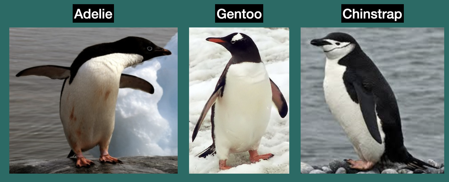
train = pd.read_csv(train_url)Classifying Palmer Penguins
In this blog post, I analyze the Palmer Penguins dataset to identify the best features for determining penguin species based on their measurements.
Classifying Palmer Penguins
Abstract
In this blog post, I analyze the Palmer Penguins dataset to identify the best features for determining penguin species based on their measurements. First, I create two figures and a table to explore the relationships between different features. Next, I utilize Scikit-learn’s feature selection methods, employing chi-squared tests to select two numerical features and one categorical feature. With these features, I train and test a logistic regression model. The model demonstrates reasonable accuracy; however, to gain a better understanding of the results, I visualize the decision regions and present a confusion matrix.st features to be used to determine the species of a penguin based on its measurements. Firstly, I create two figures and a table to analysize the relationships between features. Then I use sci-kit learns feature selection with chi-squared tests to pick 2 numerical features and 1 categorical feature. Then using those features, I train and test a logistic regression model. The model was fairly accurate but to understand the results better, I plot the decision regions and use a confusion matrix.
train.head()| studyName | Sample Number | Species | Region | Island | Stage | Individual ID | Clutch Completion | Date Egg | Culmen Length (mm) | Culmen Depth (mm) | Flipper Length (mm) | Body Mass (g) | Sex | Delta 15 N (o/oo) | Delta 13 C (o/oo) | Comments | |
|---|---|---|---|---|---|---|---|---|---|---|---|---|---|---|---|---|---|
| 0 | PAL0809 | 31 | Chinstrap penguin (Pygoscelis antarctica) | Anvers | Dream | Adult, 1 Egg Stage | N63A1 | Yes | 11/24/08 | 40.9 | 16.6 | 187.0 | 3200.0 | FEMALE | 9.08458 | -24.54903 | NaN |
| 1 | PAL0809 | 41 | Chinstrap penguin (Pygoscelis antarctica) | Anvers | Dream | Adult, 1 Egg Stage | N74A1 | Yes | 11/24/08 | 49.0 | 19.5 | 210.0 | 3950.0 | MALE | 9.53262 | -24.66867 | NaN |
| 2 | PAL0708 | 4 | Gentoo penguin (Pygoscelis papua) | Anvers | Biscoe | Adult, 1 Egg Stage | N32A2 | Yes | 11/27/07 | 50.0 | 15.2 | 218.0 | 5700.0 | MALE | 8.25540 | -25.40075 | NaN |
| 3 | PAL0708 | 15 | Gentoo penguin (Pygoscelis papua) | Anvers | Biscoe | Adult, 1 Egg Stage | N38A1 | Yes | 12/3/07 | 45.8 | 14.6 | 210.0 | 4200.0 | FEMALE | 7.79958 | -25.62618 | NaN |
| 4 | PAL0809 | 34 | Chinstrap penguin (Pygoscelis antarctica) | Anvers | Dream | Adult, 1 Egg Stage | N65A2 | Yes | 11/24/08 | 51.0 | 18.8 | 203.0 | 4100.0 | MALE | 9.23196 | -24.17282 | NaN |
Data Preparation
This code is from Professor Phil’s website. It removes unused columns and NA values, converts categorical feature columns into “one-hot encoded” 0-1 columns, and saves the resulting DataFrame as X_train. Additionally, the “Species” column is encoded using LabelEncoder and stored as y_train.
from sklearn.preprocessing import LabelEncoder
le = LabelEncoder()
le.fit(train["Species"])

def prepare_data(df):
  df = df.drop(["studyName", "Sample Number", "Individual ID", "Date Egg", "Comments", "Region"], axis = 1)
  df = df[df["Sex"] != "."]
  df = df.dropna()
  y = le.transform(df["Species"])
  df = df.drop(["Species"], axis = 1)
  df = pd.get_dummies(df)
  return df, y

X_train, y_train = prepare_data(train)
We can check what the columns look like now.
X_train.head()| Culmen Length (mm) | Culmen Depth (mm) | Flipper Length (mm) | Body Mass (g) | Delta 15 N (o/oo) | Delta 13 C (o/oo) | Island_Biscoe | Island_Dream | Island_Torgersen | Stage_Adult, 1 Egg Stage | Clutch Completion_No | Clutch Completion_Yes | Sex_FEMALE | Sex_MALE | |
|---|---|---|---|---|---|---|---|---|---|---|---|---|---|---|
| 0 | 40.9 | 16.6 | 187.0 | 3200.0 | 9.08458 | -24.54903 | False | True | False | True | False | True | True | False |
| 1 | 49.0 | 19.5 | 210.0 | 3950.0 | 9.53262 | -24.66867 | False | True | False | True | False | True | False | True |
| 2 | 50.0 | 15.2 | 218.0 | 5700.0 | 8.25540 | -25.40075 | True | False | False | True | False | True | False | True |
| 3 | 45.8 | 14.6 | 210.0 | 4200.0 | 7.79958 | -25.62618 | True | False | False | True | False | True | True | False |
| 4 | 51.0 | 18.8 | 203.0 | 4100.0 | 9.23196 | -24.17282 | False | True | False | True | False | True | False | True |
Data Visualization
Figures
I created two graphs each two quantative columns and one qualitative columns. Plot 1 shows the relationship with the body mass and flipper length between different penguin species. Plot 2 shows the difference in Culmen Length and depth across different penguin species.
# Get the unencoded columns for easier graphing.
qual = train[["Island", "Sex", "Species"]].dropna()

# Shorten species label for the legend
qual["Species"] = qual["Species"].apply(lambda x: "Chinstrap" if x == "Chinstrap penguin (Pygoscelis antarctica)"
                                         else ("Gentoo" if x == "Gentoo penguin (Pygoscelis papua)"
                                               else "Adelie"))
from matplotlib import pyplot as plt
import seaborn as sns
plt.style.use('seaborn-v0_8-whitegrid')
fig, ax = plt.subplots(1, 2, figsize = (10, 4))
p1 = sns.scatterplot(X_train, x = "Body Mass (g)", y = "Flipper Length (mm)", hue=qual["Species"], ax = ax[0])
p2 = sns.scatterplot(X_train, x = "Culmen Length (mm)", y = "Culmen Depth (mm)", hue=qual["Species"], ax = ax[1])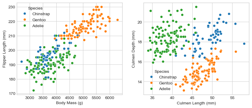
Plot 1 (Left): This graph shows the relationship between body mass and flipper length among different penguin species. Gentoo penguins are the largest, while Chinstrap and Adelie penguins overlap considerably in size. Adelie penguins show slightly more variation in mass for a given flipper length compared to Chinstraps.
Plot 2 (Right): This graph illustrates the differences in culmen length and depth among the species. Adelie penguins have the deepest but shortest culmen, Gentoo penguins have longer but less deep culmens, and Chinstraps are in between. These differences in beak size are significant for distinguishing penguin species.
Table
Now I create a summary table of the penguins measurements based on clutch completetion.
table = X_train[["Clutch Completion_Yes", "Culmen Length (mm)", "Culmen Depth (mm)", "Flipper Length (mm)", "Body Mass (g)"]]
table.groupby("Clutch Completion_Yes").aggregate(['min', 'median', 'max'])| Culmen Length (mm) | Culmen Depth (mm) | Flipper Length (mm) | Body Mass (g) | |||||||||
|---|---|---|---|---|---|---|---|---|---|---|---|---|
| min | median | max | min | median | max | min | median | max | min | median | max | |
| Clutch Completion_Yes | ||||||||||||
| False | 35.9 | 43.35 | 58.0 | 13.7 | 17.85 | 19.9 | 172.0 | 195.0 | 225.0 | 2700.0 | 3737.5 | 5700.0 |
| True | 34.0 | 45.10 | 55.9 | 13.1 | 17.20 | 21.5 | 176.0 | 198.0 | 230.0 | 2850.0 | 4100.0 | 6300.0 |
Table 1: This table shows that the most significant difference between penguins that had a full clutch and those that did not is their weight. Most of the penguins that produced two eggs weighed approximately 300 grams more. While there may be a correlation between clutch completion and weight, it is unlikely that there is a direct causation. Since clutch completion does not appear to impact this data significantly, it may not be a feature worth further investigation.
Feature selection
Here I used the SelectKBest function from the sci-kit-learn library to choose the three features that I will include in my model. I separated feature selection because all three selected features are numerical. SelectKBest identifies the k best features based on a user-specified scoring function. I chose the chi-squared scoring function, as my features are intended for classification and are non-negative
from sklearn.feature_selection import SelectKBest, chi2

# Selecting 2 numerical feature
quant = ['Culmen Length (mm)', 'Culmen Depth (mm)', 'Flipper Length (mm)', 'Body Mass (g)']
sel1 = SelectKBest(chi2, k=2)
sel1.fit_transform(X_train[quant], y_train)
f1 = sel1.get_feature_names_out()

# Selecting 1 categorical feature
qual = ["Clutch Completion_Yes", "Clutch Completion_No", "Island_Biscoe", "Island_Dream", "Island_Torgersen", "Sex_FEMALE", "Sex_MALE"]
sel2 = SelectKBest(chi2, k=1)
sel2.fit_transform(X_train[qual], y_train)
f2 = sel2.get_feature_names_out()
This function is so that I can get all the variations of the categorical feature.
def get_feat(f1, cat):
    cols = list(f1)
    clutch = ["Clutch Completion_Yes", "Clutch Completion_No"]
    island = ["Island_Biscoe", "Island_Dream", "Island_Torgersen"]
    sex = ["Sex_FEMALE", "Sex_MALE"]

    if cat in clutch: return cols + clutch
    if cat in island: return cols + island
    if cat in sex: return cols + sex
cols = get_feat(f1, f2[0])
cols['Flipper Length (mm)',
'Body Mass (g)',
'Island_Biscoe',
'Island_Dream',
'Island_Torgersen']Although the culmen sizes initially appeared to be better features, the statistical tests indicated that flipper length and body mass were, in fact, the more significant features.
Training
The model is trained on the data with features determined from above. I had to use StandardScalar to avoid a convergence error. I used the Logistic Regression model as it is a good fit for classification.
from sklearn.linear_model import LogisticRegression
from sklearn.pipeline import make_pipeline
from sklearn.preprocessing import StandardScaler


pipe = make_pipeline(StandardScaler(), LogisticRegression())
pipe.fit(X_train[cols], y_train)
pipe.score(X_train[cols], y_train)0.8984375Testing
test_url = "https://raw.githubusercontent.com/PhilChodrow/ml-notes/main/data/palmer-penguins/test.csv"
test = pd.read_csv(test_url)

X_test, y_test = prepare_data(test)
pipe.score(X_test[cols], y_test)0.8970588235294118Results
Plotting Decision Regions
Most of this code is adapted from Prof. Phil’s website.
from matplotlib import pyplot as plt
import numpy as np
from matplotlib.patches import Patch

def plot_regions(model, X, y):

    x0 = X[X.columns[0]]
    x1 = X[X.columns[1]]
    qual_features = X.columns[2:]

    fig, axarr = plt.subplots(1, len(qual_features), figsize = (8, 3))

    # create a grid
    grid_x = np.linspace(x0.min(),x0.max(),501)
    grid_y = np.linspace(x1.min(),x1.max(),501)
    xx, yy = np.meshgrid(grid_x, grid_y)

    XX = xx.ravel()
    YY = yy.ravel()

    for i in range(len(qual_features)):
      XY = pd.DataFrame({
          X.columns[0] : XX,
          X.columns[1] : YY
      })

      for j in qual_features:
        XY[j] = 0

      XY[qual_features[i]] = 1

      p = model.predict(XY)
      p = p.reshape(xx.shape)


      # use contour plot to visualize the predictions
      axarr[i].contourf(xx, yy, p, cmap = "jet", alpha = 0.2, vmin = 0, vmax = 2)

      ix = X[qual_features[i]] == 1
      # plot the data
      axarr[i].scatter(x0[ix], x1[ix], c = y[ix], cmap = "jet", vmin = 0, vmax = 2)

      axarr[i].set(xlabel = X.columns[0],
            ylabel  = X.columns[1],
            title = qual_features[i])

      patches = []
      for color, spec in zip(["red", "green", "blue"], ["Adelie", "Chinstrap", "Gentoo"]):
        patches.append(Patch(color = color, label = spec))

      plt.legend(title = "Species", handles = patches, loc = "best")

      plt.tight_layout()
Regions for training set:
plot_regions(pipe, X_train[cols], y_train)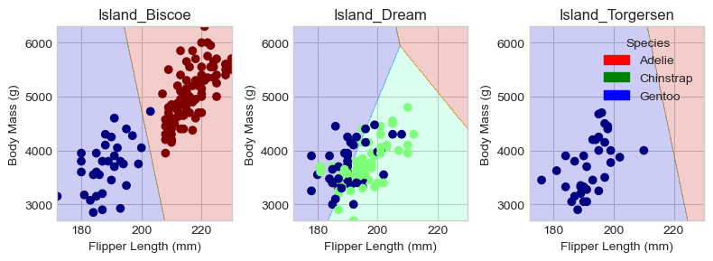
Regions for testing set:
plot_regions(pipe, X_test[cols], y_test)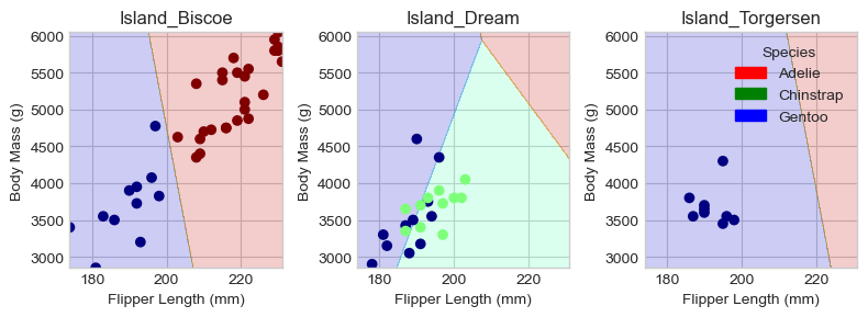
Looking at the decision plots, we can see that our model is quite successful in distinguishing between Gentoo and Adelie penguins on the Biscoe and Torgersen islands. However, on Dream Island, where there is a mixture of Gentoo and Chinstrap penguins, the model struggles to differentiate between the two species.
Confusion Matrix
from sklearn.metrics import confusion_matrix

y_test_pred = pipe.predict(X_test[cols])
confusion_matrix(y_test, y_test_pred)
array([[26, 5, 0],
[ 2, 9, 0],
[ 0, 0, 26]])Once again, this shows that model struggled the most with Gentoo and Chinstrap.
Discussion
The model achieved a training accuracy of 0.89, which is the same as its testing accuracy. This indicates that the model is quite effective at predicting penguin species based on flipper length, body mass, and island. However, the decision regions suggest that the model had difficulty distinguishing between Chinstrap and Gentoo penguins on Dream Island. It appears that these two species have similar sizes, making them challenging to differentiate.
Acknowledgements
Adapted code from Professor Phil Chodrow at Middlebury College in his class CSCI 0451: Machine Learning.